Baby Berry Reinforcement Learning Environment

If you would prefer to learn about this project by reading the code go here.

In order to revisit concepts I learned earlier in the year taking Georgia Techs fantastic graduate course in Reinforcement Learning, I decided to develop my own learning environment and solve it using a variety of RL algorithms.

Introduction to the Environment

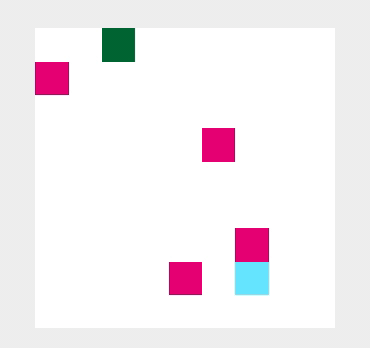
Taking inspiration from my young son who absolutely adores eating all kinds of berries, this environment is made up of a rectangular or square grid which the baby may move around attempting to collect and eat berries. The berries being spherically shaped (use your imagination below), are able to roll around the environment making the game a little more challenging for the baby. Finally, to make the task even more challenging for the intrepid berry hunter there may be a parent present marching around the grid trying to stop the baby from consuming all the expensive berries.

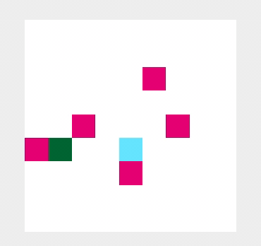
Here is an example of the baby (in blue) moving randomly around the environment. The berries (in purple) have been given a random movement probability of \(50\%\). There is a parent (in green) who is also moving randomly around the environment with probability \(50\%\). Parents (or dads as I call them in the code) are referred to as dumb if they just move randomly.

The environment is designed so that each individual berry may be given a different movement probability and starting position, or they may be assigned randomly.

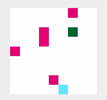
The dad may be initialized to be smart which means they move towards the baby at each time step. Here is an example of a smart dad moving again with probability \(50\%\).

The baby has a choice of five movements to take at each time step. They may move north, south, east, west or randomly. Why randomly you may be wondering. The reason a random movement is necessary is because the learners are provided with only a view of the immediate neighborhood around the baby. All algorithms were given a state size of 5 which means they can see a \(5\) by \(5\) grid with the baby in the middle. Therefore, to encourage the baby not to get stuck in an infinite loop taking the same two actions over and over a random action choice was given. However, this looping did still take place for some learners as you’ll see below.¹

Rewards are experienced by the baby at each time step. All may be set by the user but default values give a small penalty each time step for having not finished the game. A small reward for eating a berry and a large reward or punishment (negative reward) if they eat all of the berries (won the game) or are caught by the parent (game over). Finally, there is a large punishment if the baby performs an illegal move into the boundary of the board.

Programming Concepts

I used this project as an exercise in practicing my object-oriented programming. The dad class inherits the Berry methods and expands upon them. All characters are instantiated by the board and an action by the baby is handled by the board by calling methods from berries, the baby and the dad.

Some testing using assertion statements is performed when the board is initialized which helped track down some bugs when running some example environments. The whole project is neatly divided into different sections with their own folders.

Finally, I made use of type annotations and tried to write helpful docstrings so that if anyone else were to use this project it is clear what each function does.

Learning Parameters

Once the environment was created and tested it was time to solve it using a variety of RL algorithms. There are two versions of the game to beat. Both have a baby, a dad and five berries all initialized in random positions. The berries move with probability \(50\%\), the board is \(10\) by \(10\) and as outlined earlier the learners see a \(5\) by \(5\) grid with the baby in the centre. This is the current state of the board to the learner. In the easier version of the game, the dad is dumb and moves with probability \(50\%\). In the harder version, the dad is smart moving with probability \(25\%\). Any higher and the game was too difficult for the baby.

The easier game is considered beaten if the learner can average zero total reward over \(200\) consecutive episodes. In the harder game the learner has to average over \(-30\).

Finally, for the easier game the learners had \(30,000\) episodes to train over and the harder game gave \(100,000\). All the learners made use of an epsilon greedy policy for which epsilon was decayed over \(90\%\) of training episodes from \(1\) to \(0.01\).

The Learners

So far the learners successfully implemented are:

• SARSA
• \(n\)-step SARSA
• Q-learning
• Double Q-learning

All begin with an epsilon greedy policy with epsilon equal to one which means actions are chosen randomly and update Q-values based on experience playing the game until eventual convergence to the optimal policy. The convergence is guaranteed as long as all state, actions pairs are visited an infinite number of times. SARSA is the slowest to converge as the update rule

\[Q(S_t, A_t) \leftarrow Q(S_t, A_t) + \alpha (R_{t+1} + \gamma Q(S_{t+1}, A_{t+1}) - Q(S_t, A_t))\]

is the least efficient at moving towards the true Q-values.

Q-learning improves upon SARSA by updating the Q-value towards the best possible next Q-value, instead of just whatever the current policy would next select. In the update rule this translates to

\[Q(S_t, A_t) \leftarrow Q(S_t, A_t) + \alpha (R_{t+1} + \gamma \max_a Q(S_{t+1}, a) - Q(S_t, A_t))\]

As the Q-value is a measure of total discounted future reward selecting the maximum Q-value across all actions for the next state is a quicker way to update Q-values towards the optimum.

Both of these algorithms were used in the course I studied in assignments so I had experience with them already.

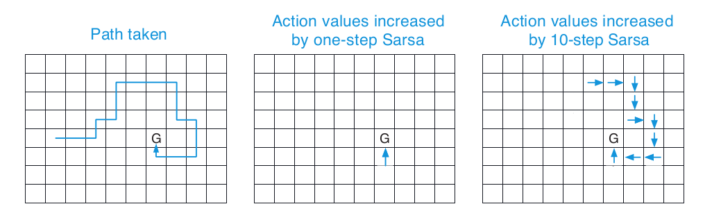
\(n\)-step SARSA is more efficient than regular SARSA (which is technically \(1\)-step SARSA) as it performs more updates to Q-values over a sample (complete episode). In the baby berry context the value of \(n\) needed to be kept low as due to the state size it did not make sense to update Q-values say ten steps before the final step when the episode ended.

A value of \(n = 3\) was found to work best in this environment which means the update rule is:

\[Q_{t+3}(S_t, A_t) = Q_{t + 3 - 1}(S_t, A_t) + \alpha (R_{t+1} + \gamma R_{t + 2} + \gamma^2 R_{t+3} + \gamma ^ 3Q_{t+2}(S_{t+3}, A_{t+3}) - Q_{t+2}(S_t, A_t))\]

The intuitive way of thinking about the algorithm is that reward experienced propagates backwards to state action pairs 3 steps previous. Sutton and Barto’s excellent book “Reinforcement Learning: An Introduction” illustrates it well on page 147

Double Q-learning makes up for a shortcoming in regular Q-learning quite elegantly. The short-come in Q-learning is most easily seen by way of a simple example. From Sutton and Barto page 135, consider the small Markov Decision Process shown below:

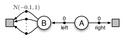
The “game” begins at state A and the player may move left or right experiencing zero reward. If the player moves right the game is over but if the play moves left they then make one more move with reward normally distributed with mean \(-0.1\) and standard deviation 1. Sometimes the reward will be positive but on average the reward should be \(-0.1\). However, during training it is entirely possible that the learner has experienced positive reward moving to the left so prefers this route. Despite the fact that on average they will experience \(-0.1\) reward and should choose to move right.

Sutton and Barton found through experiments that Q-learning chooses the left action far more frequently than it should. Double Q-learning partially alleviates this potential for maximization bias by maintaining two sets of Q values and randomly updating each one (with equal chance) at a time step. Furthermore, for each update Q-values from the other collection are used. Mathematically this means:

\[Q_1(S_t, A_t) \leftarrow Q_1(S_t, A_t) + \alpha(R_{t+1} + \gamma Q_2(S_{t+1}, \text{argmax}_a Q_1(S_{t+1}, a)) - Q_1(S_t, A_t))\]

and vice versa for updating \(Q_2\).

So those are the four algorithms currently implemented. They can be found here. I am also working on n-step Tree Backup, off-policy Monte-Carlo control, Monte-Carlo Exploring Starts and Q(\(\sigma\)) learning.

Results

Dumb Dad

All algorithms were able to beat the dumb dad except for regular SARSA. The double Q-learner was able to beat it in the fewest episodes and its running average total reward over 200 episodes is shown below.

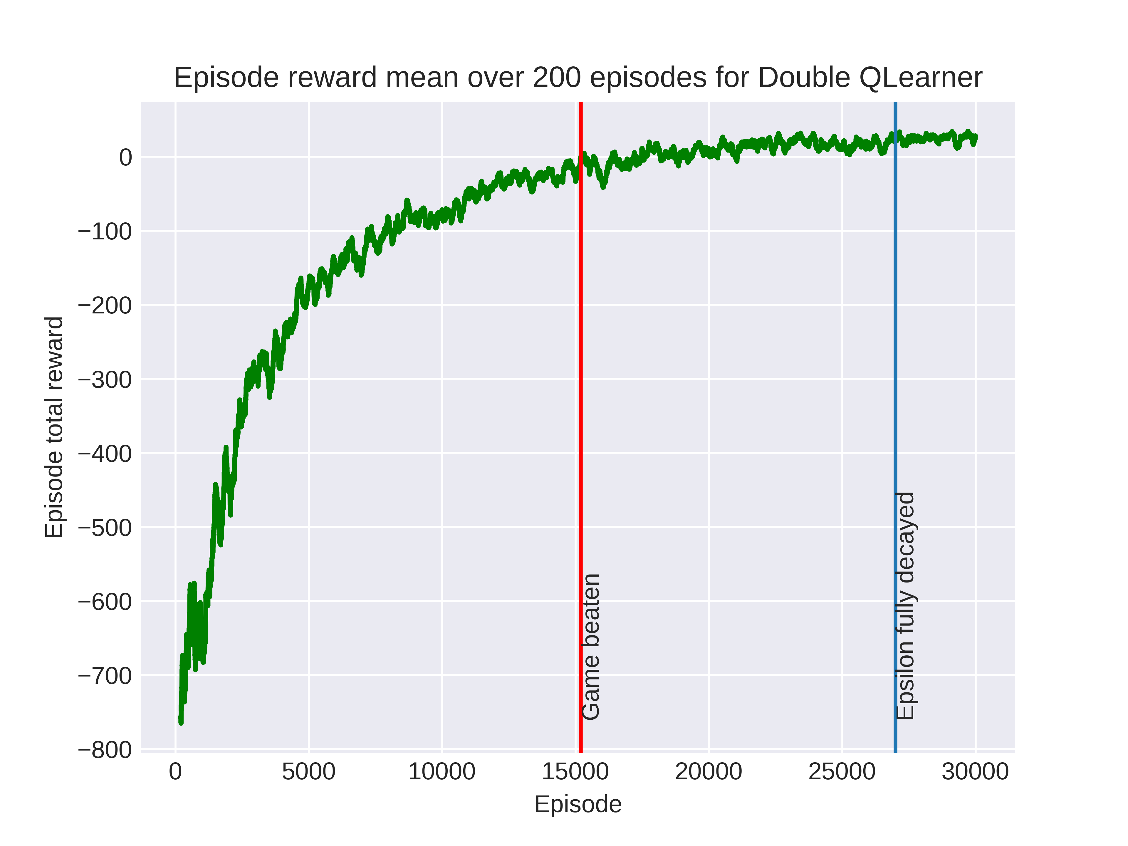
Note how training was not halted upon completion as the learner could still improve it’s strategy over the remaining episodes. Below you can see an example of the baby following the learners final policy.

You may notice that as the baby moves towards the bottom right of the grid it temporarily enters a two step loop. It would be possible to do some reward shaping and punish the learner if it enters a loop to encourage more random movement.

Smart Dad

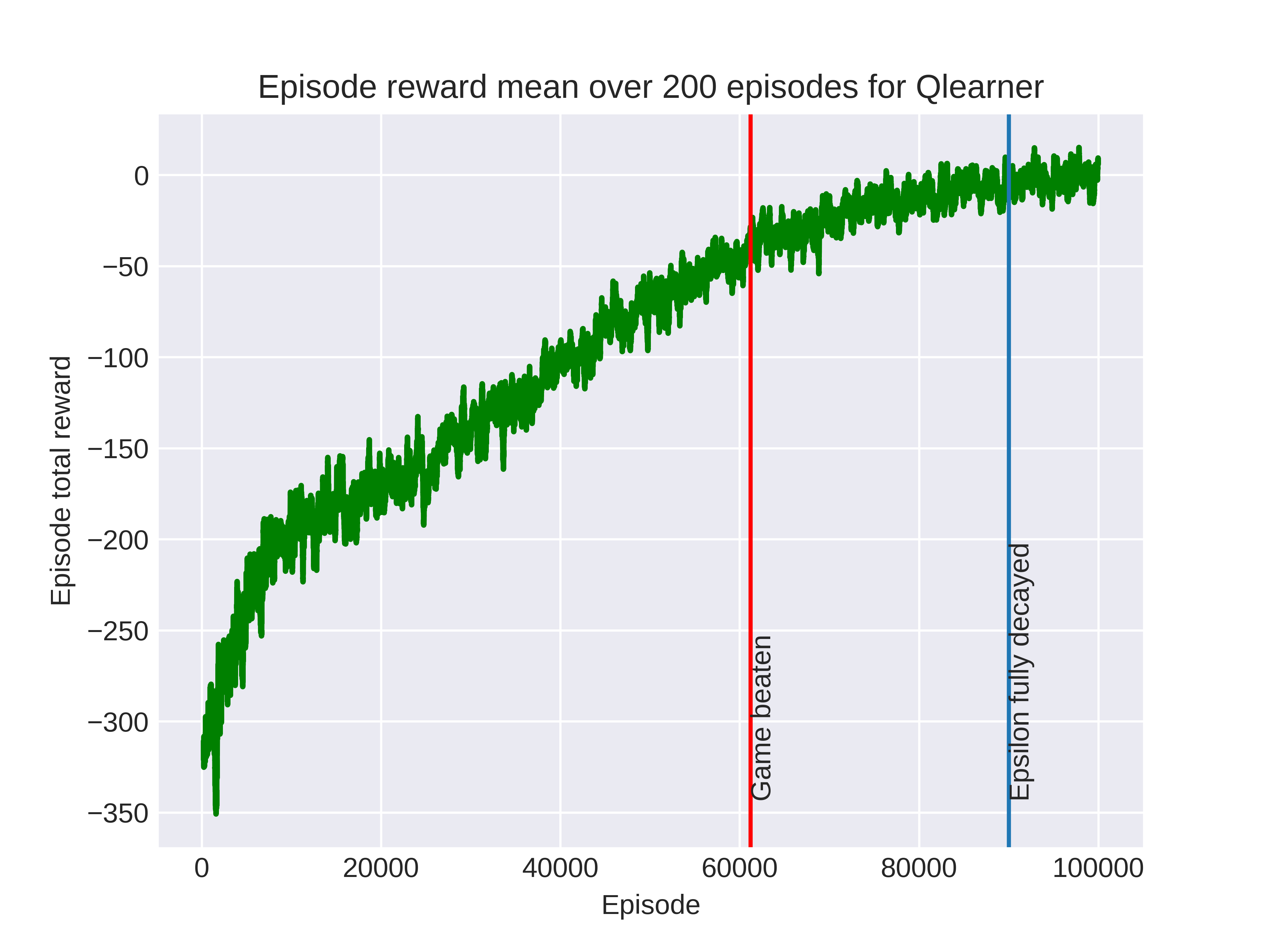
Against the smart dad, who moves towards the baby with probability 25%, the double Q-learner and Q-learner were able to beat the game in the episodes allowed (100,000). The SARSA based learners were not able to quite average -30 total reward.

Interestingly, the Q-learner outperformed the double Q-learner and its graph is shown below.

Finally, here is the Q-learner playing against the smart dad. At the beginning of the episode the baby does well to avoid the dad in the bottom right corner and then is rewarded with some berries as they move upwards. Again we can see a 2-step loop that the baby gets stuck in.

If we think about how often double Q-learner updates are performed, we notice that only half of the time each Q-value store is updated so this could explain the slower performance. For the dumb dad maybe the improvements due to avoiding maximization bias outweighed the slowdown.

What Have I Learnt?

In terms of new concepts this project has introduced double Q-learning which was not covered in the course I took. I used annotations and vertical lines in matplotlib figures for the first time. Also, creating the gifs of the game running was a new and slightly frustrating experience.

What Next?

Here is a list of additional features and algorithms I would like to add to this project.

• Finish the implementation of $n $-step Tree Backup, off-policy Monte-Carlo control, Monte-Carlo Exploring Starts and Q(\(\sigma\)) learning.
• Experiment with increasing the state view for the baby to 7.
• Add random blocks of wall to the environment.
• Change the action selection from “N”, “S”, “E”, “W”, “R” to 0, 1, 2 ,3, 4
• Fix a rare bug where the dad moves two spaces when smart.
• Add a reward penalty for getting stuck in a loop to encourage the baby to make random movements to explore the board.

1. As I was writing this I realized that in some situations the baby may want to stay still if they anticipate a berry randomly moving into them. The baby moves before the berries so maybe they would not choose to stay still but I can experiment with adding this sixth action. ↩