Melanoma Prediction Kaggle Contest - Part 2: Using Metadata

If you would prefer to go straight to the code to learn about my approach to the competition please go here. The specific notebook for the tabular models is here.

Part 1 where I introduce the contest and explore the data can be found here.

Idea

Before spending time working with the image data, a model is developed to make predictions only using the tabular data (metadata). It is not expected that this will perform particularly well but the tabular model can be emsembled with an image model to possibly give a little boost in the score. Plus these models are quick to train and give an opportunity to develop more of an intuition about the dataset.

Data Preparation

The columns that may be used for prediction with their type are:

• Sex (2 categories)
• Approximate age (numerical)
• Anatomical site on body (6 categories)
• Width of full resolution image (numerical)
• Height of full resolution image (numerical)

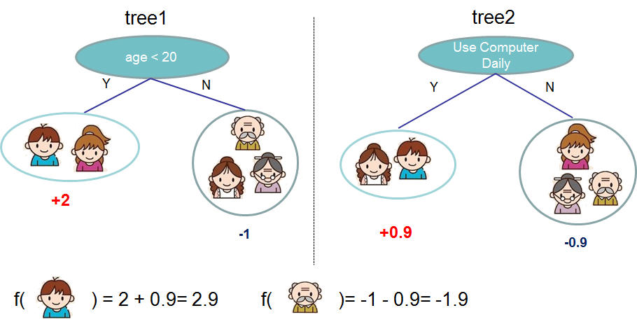
With this kind of data a gradient boosting method for classification can be a good bet. The most popular library for fitting these kind of models is XGBoost. The summary of gradient boosting is that they train many weak classifiers, most often decision trees, and then ensemble them together for better performance. A decision tree takes the form of a series of yes/no questions which result in a classification. See below for a hypothetical example for predicting whether someone will like a video game, from the XGBoost website.

This kind of model requires numerical variables so we must encode the categorical factors using dummy variables. This and other stages in the preparation of the tabular data was done in a Python file which could be neatly imported into the model training notebook.

Model Validation

As noted in the previous post, many patients had multiple entries in the training set. It was essential to make sure that patients did not exist in both training data and validation data. Fortunately, a contestant on Kaggle, Chris Deotte, graciously provided datasets where not only had he provided cross-validation folds splitting the patients but also made sure that each fold had the same proportion of malignant cases and balanced patient counts. This is referred to as triple stratified, leak-free k-fold cross validation. It is the gold-standard of cross-validation.

In the notebook, this can be seen in the extra column in all dataframes called tfrecord. It is an integer from \(0\) to \(15\) so that folds may be created by randomly splitting those integers into 1, 3 or 5 non-intersecting subsets.

The Model Pipeline

As mentioned in the previous post, there is extreme imbalance in the data where only \(1.76\%\) of data entries are malignant. To combat this a sampling strategy must be employed. To begin with, random over-sampling was used from the imblearn package. This strategy simply resamples the minority class until it makes up a designated proportion of training data.

To search for appropriate parameters for the sampler and model, scikit-learns RandomizedSearchCV was used so that \(100\) different combinations of parameters could be assessed using cross-validation. Here is the code creating the pipeline, parameters to be searched and the randomized search grid.

model_randoversamp = Pipeline([
    ('sampler', RandomOverSampler(random_state=SEED)),
    ('classification', XGBClassifier(verbosity=1, random_state=SEED))
])

params_randoversamp = {
    'sampler__sampling_strategy': [0.1, 0.3, 0.5],
    'classification__eta': [0.0001, 0.001, 0.01, 0.1, 1],
    'classification__gamma': [0, 1, 2, 3, 4, 5],
    'classification__max_depth': [x for x in range(1, 11)],
    'classification__n_estimators': [50, 100, 150, 200]
}

cv_iterator_int = []
skf = KFold(n_splits=5, shuffle=True, random_state=SEED)
for i, (idxT,idxV) in enumerate(skf.split(np.arange(15))):
    cv_iterator_int.append((train_internal.tfrecord.isin(idxT), 
                        train_internal.tfrecord.isin(idxV)))

grid_randoversamp = RandomizedSearchCV(estimator=model_randoversamp, 
                          param_distributions=params_randoversamp, 
                          n_iter=100, 
                          scoring='roc_auc', 
                          cv=cv_iterator_int, 
                          verbose=1, 
                          n_jobs=-1)

Results

This took 11.2 minutes to train on my local machine and the best performing set of parameters achieved a validation AUC-ROC of \(0.83\), which was better than I expected. This model had a sampling strategy of \(0.3\), meaning the malignant cases were resampled to bring their proportion up to \(30\%\) of the training data. The eta parameter used was \(0.1\) and this is a regularization constraint, for which larger values shrink the weights of new features added to trees. The gamma parameter chosen was 4, which is the minimum loss decrease, for a further partition to be made in a decision tree. The maximum depth of the trees chosen was 2 and this is the maximum number of decisions until a classification is made. Finally, the number of decision trees used was 100.

When this classifier was used on the test data, the classifier achieved a score of \(0.7981\) on the public Kaggle leaderboard. Impressive for a purely tabular model in my opinion. Usually, it is a big no-no to assess a model on the test set before making the final selection. However, this is a Kaggle contest and it’s nice to see how a model does on the leaderboard. More tabular models will be trained and really we should choose the best based on their performance on the cross-validated dataset before making predictions once on the test data.

A Different Sampling Strategy (SMOTE)

The next model used the same XGBoost classifier but used a more complex sampler to combat the imbalanced data.

model_smote = Pipeline([
    ('sampler', SMOTE(random_state=SEED, n_jobs=-1)),
    ('classification', XGBClassifier(verbosity=1, random_state=SEED))
])

params_smote = {
    'sampler__k_neighbors': [1, 3, 5, 7],
    'classification__eta': [0.0001, 0.001, 0.01, 0.1, 1, 10],
    'classification__gamma': [0, 1, 2, 3, 4, 5],
    'classification__max_depth': [1, 2, 3, 4, 5, 6],
    'classification__n_estimators': [100, 300, 500, 700, 900]
}

SMOTE stands for synthetic minority oversampling technique. This technique randomly selects a minority (malignant) data point and then finds \(k\) of its nearest neighbors. One of those neighbors is randomly chosen and then a new datapoint is created at a random point between the two. This new data point is a synthetic example to be fed to the model. These additional synthetic points force the decision trees to expand their decision regions which may classify the unseen validation data better.

An obvious issue is that when the minority and majority classes overlap significantly (are not separable) then these new synthetic datapoints may not be representative of the minority class. A second issue is the computation required to generate new samples. Finding \(k\)-nearest neighbors can be time exhaustive so this sampling technique is expected to take longer than random over-sampling.

The randomized search took longer this time as SMOTE sampling is more computationally expensive and as it happens, had a lower best AUC-ROC score of \(0.8218\) and \(0.7664\) on the Kaggle public leaderboard.

More Data

In an effort to improve the original randomly over-sampled model, the 2019 tabular data was added to the training data. Importantly, this external data was not included in any validation folds, only the training folds. This is because performance on external data should not be used to assess model performance. This was done by:

tf_int = train_internal['tfrecord']
tf_ext = train_external['tfrecord']
tf_ext += 20
tf = pd.concat([tf_int, tf_ext], axis=0, ignore_index=True)

cv_iterator_ext = []
skf = KFold(n_splits=5, shuffle=True, random_state=SEED)
for i, (idxT,idxV) in enumerate(skf.split(np.arange(15))):
    cv_iterator_ext.append((tf.isin(idxT) | (tf >= 20), 
                        tf.isin(idxV)))

Chris Deotte who put together the datasets found some patient entries in both the 2019 and 2020 datasets. He highlighted these with a -1 in the tfrecord column. The above code ensures these are not used for training.

The model with external data performed slightly worse than the model using just the internal data. Due to this model taking longer (17.2 minutes) than just the internal data but not giving an improved performance I decided to stick to just the internal data.

Parameter Refining

In a final effort to squeeze some increased performance out of the classifier another parameter search was used but rather than using lists, probability distributions were used with means equal to the chosen parameter from the original model. Here are the chosen parameter and the associated distribution:

• Sampling proportion 0.3 Uniform(low=0.1, high=0.5)
• Eta (regularization) 0.1 Gamma(shape=2, scale=0.05)
• Gamma (minimum loss) 4 Gamma(shape=2, scale=1)
• Maximum depth of tree 2 RandomInt(low=1, high=3)
• Number of estimators 100 RandomInt(low=50, high=150)

It should be fairly clear why the uniform and random integer distributions were used. The gamma distribution was chosen for eta and gamma, as these variables are continuous and may take values in the range \([0, \infty)\) which is the same as the gamma distributuion. It looks like a skewed normal distribution which cannot go negative which is appropriate for these variables. The mean of a gamma distribution is shape \(\times\) scale.

It took 13.4 minutes to train this model, looking at 200 possible combinations of parameters and its score on the validation data was \(0.8313\) which suggests better performance. Indeed this model did better on the Kaggle leaderboard scoring \(0.8176\).

Insight From The Model

Another great feature of gradient boosted trees, is that we may examine which variables were used most often to perform feature selection. Here is a plot of feature importance:

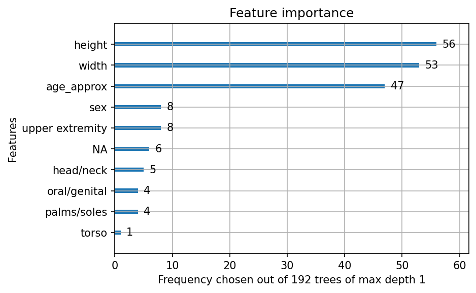
The final model had maximum depth \(1\), so the this bar plot shows which of the \(192\) estimators was based on each variable. The height and width of the original full resolution image were the best predictors, with age being the third best.

Here are some example trees:

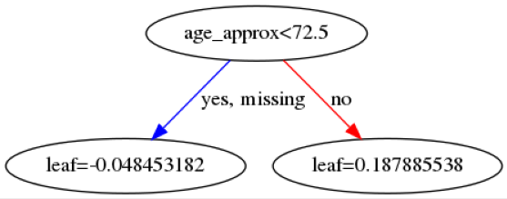
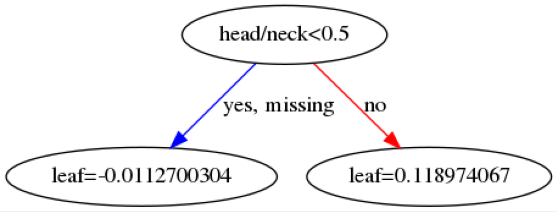
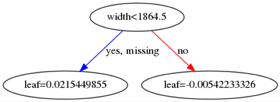
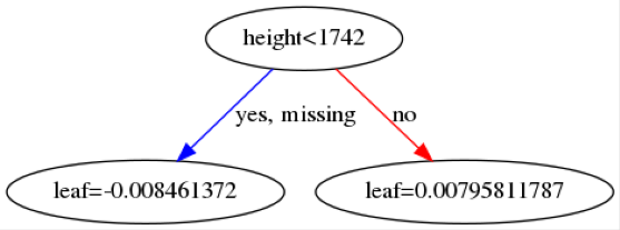
The leaf values at the bottom will be summed across all \(142\) trees and then transformed into a probability using a sigmoid function. The first image indicates that if a patient is below 72.5 years old then then this makes it more likely the patient will be predicted as benign.

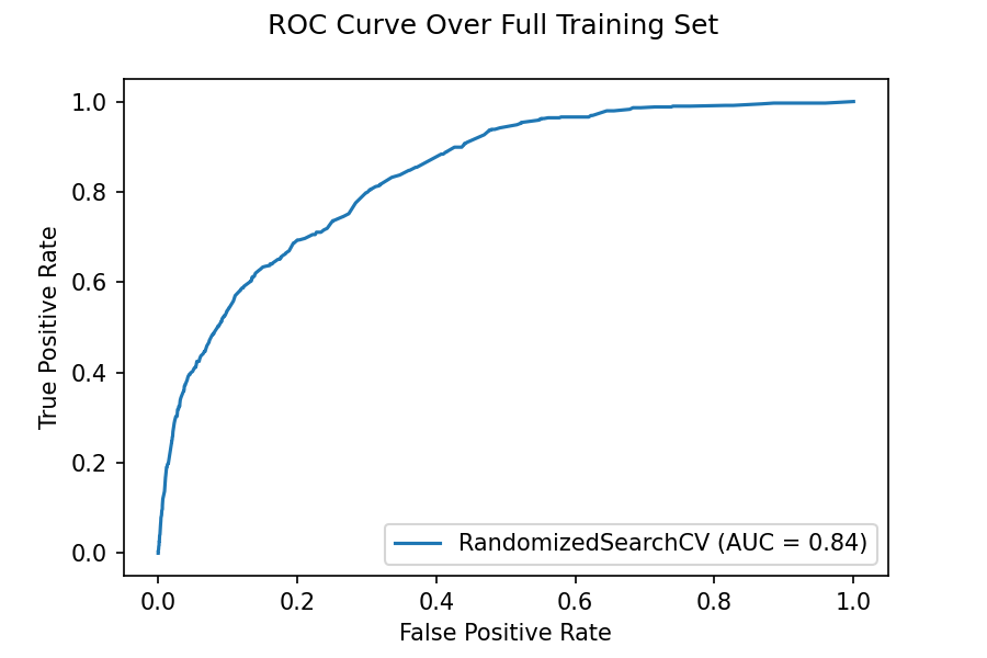
ROC Curve

Below we see the ROC curve which is found over the whole training set. The data used for the plot contains all training and validation, so we should not rely on this curve for a detailed analysis of performance of the model. However, I wanted to show this one because it has an interesting feature. Notice how the curve asymptotes very close to a horizontal line for large values on the \(x\)-axis and it asymptotes not as close to the vertical for low values on the \(x\)-axis. This makes sense for our data as we have much less positive data than negative. So it is easy to achieve a high true positive rate by putting the threshold very high so only points that the model is extremely sure of being malignant are classed as so. However, it is hard to keep the false positive rate low because there are so few positives the model is sure to misclassify negatives as positives for low thresholds.

What Have I Learnt?

Here is a list of the techniques, technologies, concepts completing this project has introduced to me for the first time.

• Randomized grid search over probability distributions in scikit-learn
• Using an XGBoost classifier to perform feature selection
• The surprising ability for solely tabular patient data to predict melanoma
• Different sampling techniques using the imblearn library