Melanoma Prediction Kaggle Contest - Part 3: Image Data

If you would prefer to go straight to the code to learn about my approach to the competition please go here. The notebooks for the models on this page can be found here.

Previously: Part 1 and Part 2.

Big thanks: the user Roman has provided many public notebooks on Kaggle which were incredibly useful in developing my own code for this contest. I cannot find (because they have so many) the original notebook which inspired me most but check out their work on Kaggle.

Introduction

It is now time to train models which will use the patient image data. As we are making predictions using images, we will be using convolutional neural networks. I begin training some smaller models which can be done on my local machine and then test out training a larger model before sending the computation to the cloud so that larger image sizes can be used.

Image Augmentations

It is a almost always a good idea to perform augmentations on the images before passing them to the model for training. This diversifies and increases the size of the training data and should help the model to generalize to more varied images. Augmentations should be used that are appropriate to the training set. If you are trying to classify images of dogs into different breeds then it would not make sense to reflect an image across the horizontal because you will not need to classify pictures of upside down dogs.

The code for my image augmentations can be found here. The augmentations used were:

• Horizontal flip
• Vertical flip
• Shear in X
• Shear in Y
• Translate in X
• Translate in Y
• Rotation
• Apply auto-contrast
• Apply equalization (equalizes the histogram of the image to create a uniform distribution of greyscale pixels)
• Solarize (inverts all pixels above a certain threshold)
• Posterize (reduces the number of bits for each pixel)
• Change contrast
• Color balance (similar to settings on a television)
• Brightness
• Sharpness
• Cutout (cuts out a rectangular shape and fills with a fill-color)

The images to be classified are photos of skin lesions taken directly from above. So most augmentations make sense as there is no fixed perspective.

The next thing to decide is how many of these to be applied and what parameters to be used with them. For example, by how many degrees do we rotate and how often? I followed the advice from the paper UniformAugment: A Search-free ProbabilisticData Augmentation Approach. The key takeaway from this paper is that, “a uniform sampling over the continuous space of augmentation transformations is sufficient to train highly effective models”. With this is mind, to get an image from the training data to be passed to the network, a random sample of two augmentations was chosen from all that are possible above. Then each was performed uniformly at random with a magnitude randomly chosen from their range of possible magnitudes. Here is the code that explains how this happens exactly:

def __call__(self, img: PIL.Image) -> PIL.Image:
"""
Select a random sample of augmentations where 
`self.operations` determines how many and perform them
on the image
"""
    operations = random.sample(list(self.augs.items()), self.operations)
    for operation in operations:
        augmentation, range = operation
        # Uniformly select value from range of augmentations
        magnitude = random.uniform(range[0], range[1])
        # Perform augmentation uniformly at random
        probability = random.random()
        if random.random() < probability:
            img = self.func[augmentation](img, magnitude)
    return img

To show this in action, here is a sample of 20 images with their augmentations. Remember some of these will have no augmentation at all. These are the not the exact form of the images that are passed to the model, as they have not been normalized according to the ImageNet databases mean and standard deviation. Almost all pre-trained neural networks are trained on this dataset, so images should be normalized according to the same summary statistics. If I was to show normalized images they would be bright, garish colors.

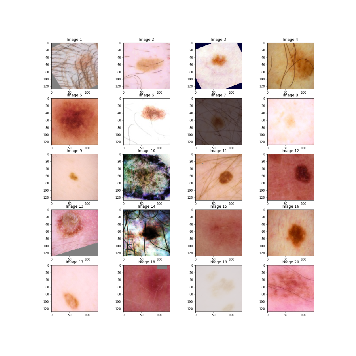
We can see in image 1 a rotation. In image 3, a rotation and an auto-contrast. Image 7 is an example where the brightness has been altered. Both images 10 and 14 have been equalized. Finally, image 18 has a small cutout in the top right corner.

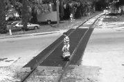
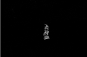
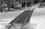
A few more advanced image augmentations which I did not use but would like to try in the future are either adding hairs to non-hair images or using robust principal component analysis to remove the hairs from the foreground. I used this method in a Georgia Tech class to remove a person from the foreground of an image like below:

Original image

Foreground (person) isolated

Person removed from original image to leave background

Finally, some of the images are circular suggesting that they are from a microscope. Randomly making images circular could be an augmentation to increase performance.

Software

I will be using PyTorch for the CNN model implementation. The Python file where I create the networks and key functions required for training can be found here. Torchvision and PIL are used for image augmentations. Finally, the models are trained using a standard process in notebooks, here is a ResNet example.

Model Parameters

Despite using a relatively standard training, validation and testing strategy with fairly standard architectures, there are still a number of parameters to be chosen. My choices with justification come next.

Model Architecture

The architectures that I used on my local machine were AlexNet and ResNet18. These are fairly small convolutional neural networks, in the sense of the number of parameters to be trained. Once I moved the computation to the cloud, I used EfficientNets. I will briefly explain the idea behind them from the paper EfficientNet: Rethinking Model Scaling for Convolutional Neural Networks. The authors, Mingxing Tan and Quoc V. Le, performed an architecture search where they scaled the three main measurements that determine the size of a network using the same scaling constant. The three dimensions of convolutional neural networks they scaled were:

• Width: the number of channels of each layer in the CNN
• Depth: the number of layers in the CNN
• Resolution: this is effectively the size of the images fed into the model

By first finding an efficient baseline network EfficientNet-B0 (based on MobileNetV2), they then scaled it larger and larger to achieve greater performance on ImageNet, using constants for each of width, height and depth in a principled way. Their baseline network EfficientNet-B0 has around one fifth the number of parameters as ResNet-50 but higher accuracy. As a result of their paper, they found EfficientNet architectures from B0 to B7 increasing in size and accuracy. For example, EfficientNet-B7 has around one eighth the number of parameters as GPipe, the previously best performing CNN on ImageNet, yet outperforms it to achieve at the time state of the art performance.

So EfficientNets are not only more efficient than other networks commonly used, they are often more accurate. This made them a common choice in the competition amongst competitors.

Batch Size

This is the number of images sent to the network together for training. Generally, the higher the batch size the better so I sent as many could be handled by the GPU or CPU at once. For the larger networks I trained this had to be either 16 or 32 images.

Loss Function

As this is a binary classification problem I used Cross Entropy loss which has the following formula

\[H = - \frac{1}{N} \sum_{i=1}^N \left[ y_i \log \hat{y}_i+ (1 - y_i) \log (1 - \hat{y}_i) \right]\]

where \(y_n\) is the true label of y (\(0\): benign, \(1\): malignant), \(\hat{y}_n\) the predicted probability of \(y\) being malignant and \(N\) the number of total images in the loss calculation. This loss function punishes high \(\hat{y}\) values when the actual label is \(0\) and vice-versa.

Optimization

I use the Adam algorithm for stochastic optimization. It is both computationally efficient and has little memory requirements. This is the most common optimization algorithm used in neural network training.

Learning Rate

An initial learning rate of 1e3 \(= 0.001\) is used but it is scheduled to decrease once the validation accuracy plateaus. This is implemented in PyTorch using

optimizer = optim.Adam(net.parameters(), lr=1e3)
scheduler = ReduceLROnPlateau(optimizer=optimizer, mode='max', patience=2, factor=0.2)

where mode='max' means the learning rate will be decreased once the validation accuracy stops increasing, patience=2 means we will allow only 2 epochs of non-increasing performance and factor=0.2 means the current learning rate will be multiplied by \(0.2\) for the decrease. Another learning rate scheduler which performs well is cyclic learning rates which is also available in PyTorch.

Sampling

I use the WeightedRandomSampler from PyTorch to ensure the minority class (malignant) is sampled often enough to make sure it is \(50\%\) of the training data. It is possible that it would be better to only sample until it makes up maybe \(20\%\) of the data but I did not have enough time (and compute) to try this. I also wanted to use SMOTE with the image data but could not find a PyTorch implementation.

Number of Epochs

For the local smaller networks I trained for 10 epochs and for the cloud ones 20. This was purely due to time and computation limits. I would have trained for longer if I had access to better hardware. I experimented with larger ResNet models which could fit into my laptops memory but I could not train for enough epochs and the models were under-fit.

Frozen Epochs

I left all layers of the models, except the final, frozen for the first 3 epochs. This is because I was using pre-trained networks which have had their final layer changed to match the cancer prediction binary classification problem, rather than the ImageNet classification problem. The networks are pre-trained on ImageNet which contains images of all manner of different objects/animals/things. By freezing all but the last layer, we can relatively quickly get good performance on the cancer image data and them unfreeze the full network and train the lower layers to the specific task. This is called transfer learning.

Early Stopping

This technique is to combat over-fitting by stopping training if an increase in performance on the validation set is not found for a certain number of epochs in a row. I had this set to 3 for the local training and 5 for cloud training. This way a reduction in the learning rate can be tested, and then training halted if better performance is not experienced with the lower learning rate.

Test Time Augmentations

It is common with computer vision tasks where augmentation is performed on training data to also perform the augmentation on the test data when making final predictions. By feeding the same test image multiple times with different augmentations the predictions can be averaged. The idea is that by doing this the error in the prediction is averaged and large errors which effect final accuracy are lowered. For local training I performed 3 test time augmentations, for the cloud training I performed 10. These take a long time so for a real-world application where predictions need to be as fast as possible, they may not be practical.

Model Assessment

As with the tabular data, triple-stratified leak free k-fold cross validation will be used. Thanks again to Chris Deotte for creating the folds! When I had more time and compute, I used 5-fold cross-validation but when I was low on time and compute I used 3-fold. When external data was used it was only added as training data.

The metric used for validation is AUC-ROC as this is the metric to be assessed by Kaggle.

Cloud Compute

Once I started to train the larger models it was completely infeasible to use my laptop. Before this Kaggle contest I was studying the fast.ai course “Deep Learning for Coders” and had signed up for Google Cloud Platforms introductory $300 of cloud compute. I used this to train the models until it ran out. My final big model trained was an EfficientNet-B2 using 384 \(\times\) 384 size images and all of the 2019 external data. For this final model I had to train it on Google colab. This posed challenges as their free GPU usage is time limited. I trained folds separately overnight using a JavaScript script to move the cursor and click a button which pops up when you are inactive. This was a painful process but beat spending my own cash on compute. It paid off as this was my best performing model, as can be seen below.

Results

Model	Local or Cloud	Image Size	External Data	CV AUC-ROC	Private LB	Public LB	Training Time (hours)
AlexNet	Local	128	No	0.7699	0.8736	0.8786	2.86
ResNet18	Local	64	No	0.8056	0.8801	0.8780	3.50
EfficientNet-B0	Cloud (GCP)	256	No	Unknown	0.9272	0.9117	Unknown
EfficientNet-B5	Cloud (GCP)	256?	Malignant only	Unknown	0.8855	0.8943	Unknown
EfficientNet-B2	Cloud (GCP)	256	Yes	0.9067	0.9277	0.9161	Unknown
EfficientNet-B2	Cloud (GCP + Colab)	384	Yes	Unknown	0.9309	0.9164	8.17

Unfortunately, I was not diligent saving statistics about all the models I trained. I often got excited to try something new and forgot to record the training that had just taken place. This is something I will improve in the future!

In this Kaggle contest, and I assume all others, before the deadline is reached only 30% of your submission is assessed to provide your score on the public leader-board. Once the deadline is reached your 3 chosen submissions are assessed on the other 70% of the test data and your private leader-board position is revealed. On the public leader-board there were multiple submission with AUC-ROC score 0.97+ but the winning submission of the contest achieved 0.9490 on the private leader-board. This team jumped 886 places from public to private!

My final position was 1538th out of 3319 competitors and my jump from public to private was 256 places. I am happy to have finished in the top half of competitors in my first Kaggle contest using only freely available computation.

The Ensembled Model

Before the final submission I was only able to ensemble one of my CNN models with my XGBoost tabular classifier. It was the ResNet18 trained on 64 \(\times\) 64 images. The notebook to find the ensemble ratio can be viewed here. By trying out proportions from 10% all the way to 90% for the tabular contribution to the prediction on the validation data, I found that the best split was 40% tabular and 60% CNN. This model achieved a supremely impressive AUC-ROC of 0.9035 on the private leader-board. I was surprised a model trained on such small images could achieve such a high score. This whole model was trained on my relatively low spec, three-year-old laptop! This model alone would have placed around 1900th out of 3300 competitors.

If I have time I would like to try ensembling the tabular model with the best performing EfficientNet model. I have the model parameters for each of the folds saved in state dictionary, so this is still possible. It would interesting to see if the tabular model is able to boost the CNN model in any way.

Extensions

If I had unlimited compute and more time there are so many more ideas I have for this contest. Here are some of them:

• Train the largest EfficientNet, on the largest images, for as many epochs as possible with 5-fold cross validation. Then ensemble this with a tabular model
• Find more external data to train the model on. Competitors gave more in the Kaggle forums
• Experiment with both adding hairs and removing them from the training data
• Instead of fitting to the benign/malignant binary, fit to the diagnosis. I can’t take credit for this, the eventual winners did this
• Train many large CNNs on large image sizes and then ensemble them to get predictions
• Use a cyclic learning rate schedule rather than the reduce on plateau I used. We used cyclic learning rates in the fast.ai course and I know Jeremy Howard is a big proponent
• Learn how to distribute training over multiple GPUs and then how to use a TPU and then multiple TPUs!
• Rather than choosing the parameters outlined earlier in this post, I found do some kind of hyper-parameter search, probably Bayesian.

Analysis Of The Winning Method

The winning team have graciously outlined on the forums what approach they took to the problem. I have summarized it below.

• Used 2018, 2019 and 2020 data for training and validation. They checked and found the cross-validation score to be more stable when using all data for validation
• They ensembled many models together. They found the more they ensembled, the higher the correlation between their cross-validated score and the leader-board score
• They trained CNN models with and without metadata. There are ways to include metadata in images
• They predicted diagnosis, rather than simply benign/malignant. This meant mapping the external diagnosis column to the 2020 version
• They used a long list of random augmentations (probability \(50\%\) of being done) and then one of some subgroups of augmentations. How they chose these is not clear
• They did not augment validation data

What Have I Learnt?

• Image augmentations are important for training CNNs and there can be very creative
• Uniform augmentations can be a way to perform augmentations which does not require much parameter tuning
• How to perform weighted sampling and use a learning rate scheduler in PyTorch
• How to use a learning rate scheduler in PyTorch
• I need to be more systematic in how I record and store my experiments
• I need to be more careful how to use cloud compute. I was careless training too many models and did not make the most of the free Google cloud credits
• That PyTorch has many pre-trained networks built in which can be loaded easily. Hopefully they add EfficientNets to these soon
• That as far as I can tell there is no SMOTE sampling implementation for PyTorch, maybe I should write one